Tag: Baumol
Overcoming Baumol
One way to overcome the Baumol effect is to replace labor with capital. AI and robots are making that possible. Here’s a clip of the Carmelite Monks of Wyoming who are building a monastery in the Gothic style using CNC machines:
CNC machines and robots have unlocked the ability to relatively quickly carve the intense details of a Gothic church. Ornate pieces that used to take months for a skilled carver, now can be accomplished in a matter of days. Instead of cutting out the beauty, using the excuse that it takes too long, thus doesn’t fit into the budget, modern technology can be used to make true Gothic in all its beauty a reality again today.
Bring back the beauty!
The Economist covers Why Are the Prices So D*mn High?
The Economist does a very nice job covering Why Are the Prices So D*mn High.
Baumol’s earliest work on the subject, written with William Bowen, was published in 1965. Analyses like that of Messrs Helland and Tabarrok nonetheless feel novel, because the implications of cost disease remain so underappreciated in policy circles. For instance, the steadily rising expense of education and health care is almost universally deplored as an economic scourge, despite being caused by something indubitably good: rapid, if unevenly spread, productivity growth. Higher prices, if driven by cost disease, need not mean reduced affordability, since they reflect greater productive capacity elsewhere in the economy. The authors use an analogy: as a person’s salary increases, the cost of doing things other than work—like gardening, for example—rises, since each hour off the job means more forgone income. But that does not mean that time spent gardening has become less affordable.
It’s an implication of the Baumol effect that everyone ends up working in a low productivity industry!
The only true solution to cost disease is an economy-wide productivity slowdown—and one may be in the offing. Technological progress pushes employment into the sectors most resistant to productivity growth. Eventually, nearly everyone may have jobs that are valued for their inefficiency: as concert musicians, or artisanal cheesemakers, or members of the household staff of the very rich. If there is no high-productivity sector to lure such workers away, then the problem does not arise.
Misunderstanding the Baumol effect can lead to a cure worse than the “disease”:
These possibilities reveal the real threat from Baumol’s disease: not that work will flow toward less-productive industries, which is inevitable, but that gains from rising productivity are unevenly shared. When firms in highly productive industries crave highly credentialed workers, it is the pay of similar workers elsewhere in the economy—of doctors, say—that rises in response. That worsens inequality, as low-income workers must still pay higher prices for essential services like health care. Even so, the productivity growth that drives cost disease could make everyone better off. But governments often do too little to tax the winners and compensate the losers. And politicians who do not understand the Baumol effect sometimes cap spending on education and health. Unsurprisingly, since they misunderstand the diagnosis, the treatment they prescribe makes the ailment worse.
My only complaint is that the excellent reviewer has not followed our lead and called it the Baumol effect–cost disease is a misleading name!
Addendum: Other posts in this series.
The Baumol Effect
After looking at education and health care and doing a statistical analysis covering 139 industries, Helland and I conclude that a big factor in price increases over time in the rising price of skilled labor. Many industries use skilled labor, however, and even so prices decline so that cannot be a full explanation. Moreover, why is the price of skilled labor increasing? The Baumol effect answers both of these questions. In this post, I’ll explain the effect drawing from Why Are the Prices so D*mn High.
The Baumol effect is easy to explain but difficult to grasp. In 1826, when Beethoven’s String Quartet No. 14 was first played, it took four people 40 minutes to produce a performance. In 2010, it still took four people 40 minutes to produce a performance. Stated differently, in the nearly 200 years between 1826 and 2010, there was no growth in string quartet labor productivity. In 1826 it took 2.66 labor hours to produce one unit of output, and it took 2.66 labor hours to produce one unit of output in 2010.
Fortunately, most other sectors of the economy have experienced substantial growth in labor productivity since 1826. We can measure growth in labor productivity in the economy as a whole by looking at the growth in real wages. In 1826 the average hourly wage for a production worker was $1.14. In 2010 the average hourly wage for a production worker was $26.44, approximately 23 times higher in real (inflation-adjusted) terms. Growth in average labor productivity has a surprising implication: it makes the output of slow productivity-growth sectors (relatively) more expensive. In 1826, the average wage of $1.14 meant that the 2.66 hours needed to produce a performance of Beethoven’s String Quartet No. 14 had an opportunity cost of just $3.02. At a wage of $26.44, the 2.66 hours of labor in music production had an opportunity cost of $70.33. Thus, in 2010 it was 23 times (70.33/3.02) more expensive to produce a performance of Beethoven’s String Quartet No. 14 than in 1826. In other words, one had to give up more other goods and services to produce a music performance in 2010 than one did in 1826. Why? Simply because in 2010, society was better at producing other goods and services than in 1826.
The 23 times increase in the relative price of the string quartet is the driving force of Baumol’s cost disease. The focus on relative prices tells us that the cost disease is misnamed. The cost disease is not a disease but a blessing. To be sure, it would be better if productivity increased in all industries, but that is just to say that more is better. There is nothing negative about productivity growth, even if it is unbalanced.
In this post, I will discuss some implications of the fact that productivity is unbalanced. See the book for more discussion and speculation about why productivity growth is systematically unbalanced.
The Baumol effect reminds us that all prices are relative prices. An implication is that over time prices have very little connection to affordability. If the price of the same can of soup is higher at Wegmans than at Walmart we understand that soup is more affordable at Walmart. But if the price of the same can of soup is higher today than in the past it doesn’t imply that soup was more affordable in the past, even if we have done all the right corrections for inflation.
We can see this in the diagram at right. We have a two-good economy, Cars and Education. The production possibilities frontier shows all the combinations of Cars and Education that we can afford given our technology and resources at time 1 (PPF 1). Now suppose society chooses to consume the bundle of goods denoted by point (a). The relative price of Cars and Education is given by the slope of the PPF at that point. That price/slope tells us if we give up some education how many more cars can we get? In a market economy the price has to be given by the slope of the PPF because that is the only price at which people will willing consume the bundle of goods at point (a), i.e. it’s the equilibrium price.
Now at time 2, productivity has increased which means that with the same resources we can now have more of both goods. Productivity of Car production has increased more than that of Education production, however, so the curve shifts out more towards Cars than towards Education. Suppose society continues to consume Cars and Education in the same proportions, i.e. at point (b). The price of education must increase–and all that means is that if we give up a unit of education at point b we will get more cars than before which is the same as saying that if we want more education at point b we must give up more cars than before, i.e. the price has increased.
Notice, however, that although the price of education has increased, education is not less affordable. Indeed, at point (b) we are consuming more of both goods–broadly speaking this is exactly what has happened–namely, the price of education has increased and we now consume more of it than ever before.
When we recognize that all prices are relative prices the following simple yet deep facts follow:
- If productivity increases in some industries more than others then, ceteris paribus, some prices must increase.
- Over time, all real prices cannot fall.
In Figure 22 the economy moves from point (a) to point (b). If we graph the same transition over time it will look something like Figure 23.
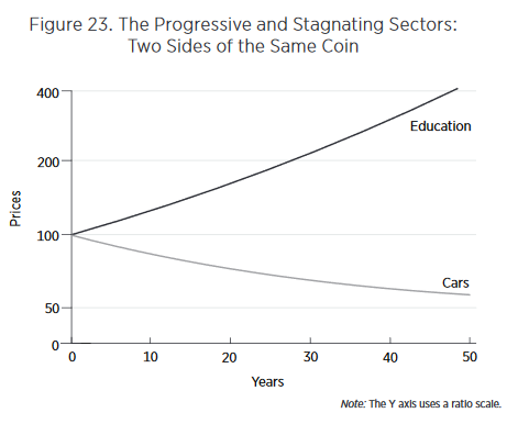
Looking at such graphs, our attention naturally is drawn to the rising cost of education. Why are costs rising so quickly? Entranced by such graphs, we may enter into a detailed analysis of the special factors of education—regulation, unionization, government purchases, insurance, international trade, and so forth—to try to explain the dramatic increase in costs. Yet the rising costs in the education sector are simply a reflection of increased productivity in the car sector. Thus, another deep lesson of the Baumol effect is that to understand why costs in the stagnant sector are rising, we must look away from the stagnating sector and toward the progressive sector.
Finally, there is one other addition to the Baumol effect which is not often recognized but worth drawing attention to. In Figure 22, I assumed that preferences were such that people wanted to consume the same ratio of goods over time so we moved from point (a) to point (b). But suppose that as we get wealthier we get tired of more cars and would like relatively more education so we move towards point (d). As we move from point (b) to point (d) we are taking resources away from car production, resources which were probably well-suited to making cars, and instead moving them towards education where they are probably less well suited. As a result as we move from point (b) to point (d) we are driving up the price of education as we try to turn auto workers into teachers. In this case, the Baumol effect gets magnified. We could alternatively move from point (b) to point (c) which would turn teachers into less productive auto workers thus driving down the price of education (i.e. increasing the price of cars). Thus, depending on preferences, the Baumol effect can be magnified or ameliorated.
As a society it appears that with greater wealth we have wanted to consume more of the goods like education and health care that have relatively slow productivity growth. Thus, preferences have magnified the Baumol effect.
Next week, I will wrap up the discussion by explaining some features of the data that the Baumol effect fits much better than do other theories.
Addendum: Other posts in this series.
Why Are the Prices So D*MN High?
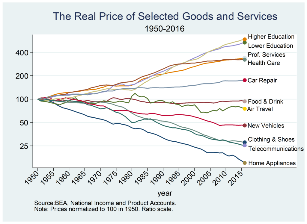
Why have some prices increased since 1950 by a factor of four while other prices have decreased by a factor of four? Technology is making so many goods and services much cheaper than in the past–that seems to be the normal situation–so why do some industries seem not only to be not progressing but actually retrogessing? As Scott Alexander put it, why are some industries so weird?
Those are the questions that motivated my latest piece, a short book with Eric Helland just released by the Mercatus Center titled, Why are the Prices so D*mn High?
In approaching this question I had some ideas in mind. I assumed that regulation, bloat and bureaucracy, monopoly power and the Baumol effect would each explain some of what is going on. After looking at this in depth, however, my conclusion is that it’s almost all Baumol effect. That conclusion radically changes one’s evaluation of price increases and decreases over the long run and it changes what, if anything, one might try to do to address such price changes.
Next week I will examine some of the evidence that pushes me towards this verdict. I’ll also take a closer look at the Baumol effect, which is mistakenly called the cost disease.
Let’s note here, however, what we need to explain. For the most part, we don’t see quick, big changes in prices that then level off. That in itself is interesting since policy tends to be discontinuous. We might expect a big regulation, for example, to cause a big increase in prices as industries adjust but then growth should return to normal. Instead, what we see and need to explain is slow, steady rising relative prices that happens over decades. Indeed, in some cases, such as education, prices have been increasing faster than average for more than a century! Puzzle over that over the long weekend. More next week!
Addendum: Other posts in this series.